Location Intelligence
Location intelligence is based on the idea that geographical spaces are a particular analytical dimension in the BI domain. It is based on:
- the geographical representation of data,
- interaction with GIS systems,
- spatial data,
- spatial operators.
Location Intelligence usually guarantees:
- an immediate perception of a phenomena distribution over a geographical area,
- interactivity,
- multivariate analysis,
- temporal snapshots.
Location Intelligence is becoming widely used, mostly thanks to the emergence of location services such as Google Maps. This domain is very easy to use for all kinds of users, usually analysts and operational profiles. By contrast, its management is not as easy, especially if it implies an internal management of the geographical data base.
Basic concepts
The term Location Intelligence refers to all those processes, technologies, applications and practices capable to join spatial data with business data, in order to gain critical insights, to better support decisional processes and to optimize business activities.
At the technological level, this correlation is the result of the integration between the software systems that manage these two heterogeneous types of data: geographic information systems (GIS), which manage spatial data, and Business Intelligence systems (BI), which manage business data. This integration gives rise to new technological tools supporting decision-making processes, and the analysis on those business data that are directly or indirectly related to a geographic dimension.
Location Intelligence applications significantly improve the quality of users’ analysis based on a geographic dimension. Indeed, a Data Warehouse (DWH) almost always included such information. By representing the geographic distribution of one or more business measures on interactive thematic maps , users can quickly identify patterns, trends or critical areas, with an effectiveness that would be unfeasible using traditional analytical tools.
More on GIS and Spatial Data*
Spatial Data
The term spatial data refers to any kind of information that can be placed in a real or virtual geometric space. In particular, if the spatial data is located in a real geometric space — which is a geometric space that models the real space — it can be defined as geo-referenced data.
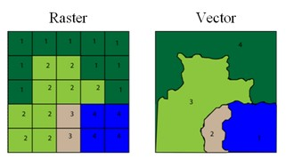
Fig. 378 A base layer in raster and vector format.
Spatial data are represented through graphical objects called maps. Maps are a portrayal of geographic information as a digital image file suitable for display on a computer screen.
According to the Open Geospatial Consortium (OGC) definition, a map is made of overlapping layers: a base layer in raster format (e.g. satellite photo) is integrated with other layers (overlays) in vector format. Each overlay is made of homogeneous spatial information, which models a same category of objects, called features.
A feature is called geographic feature when the constituting objects are abstractions of real-world physical objects and can be located univocally within a referencez coordinate system, according to their relative position.
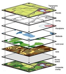
Fig. 379 Overlapping layer.
A feature includes:
- a set of attributes that describes its geometry (vector encoding). Geometric attributes must describe its relative shape and position in an unambiguous way, so that the feature can be properly drawn and located on the map, according to the other features of the layers.
- a set of generic attributes related to the particular type of physical object to be modeled. Generic attributes are not defined: they vary according to the type of abstraction that users want to give to each real-world physical object.
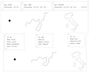
Fig. 380 Examples of feature.
There is a wide range of standards that can be used for the vector encoding of spatial data (e.g. GeoJSON, GML, Shape File, etc.). Most geographic information systems can perform the needed conversions among various encodings.
GIS
Geographic Information Systems (GIS) provide a set of software tools designed to capture, store, extract, transform and display spatial data [2]_ . Therefore, the term GIS refers a set of sole technological components that manage the spatial data during its whole life cycle, starting from the capture of the data up to its representation and re-distribution.
From a logical point of view, the key functionalities of a GIS do not differ from those of a BI system. Both systems are characterized by some specific components supporting the effective storage of data, some others supporting their manipulation, their re-distribution or their visualization. On the other hand, the implementation of these functionalities deeply differs between GIS and BI systems, since they deal with two different types of data (alphanumeric and spatial data).
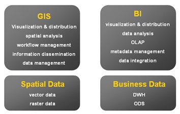
Fig. 381 Definition of GIS, BI, spatial data and business data.
Unlike the market of BI suites, the market of GIS is characterized by a wide spread of open standards, adopted by all main vendors, which regulate the interaction among the various components of the system at all architectural levels.
Note
Open Gesospatial Consortium (OGC)
The most important International organization for standardization in the GIS domain is the Open Geospatial Consortium (OGC), involving 370 commercial, governmental, non-profit and research organizations. Read more at www.opengeospatial.org.
As for the integration between GIS and BI systems, the OGC has defined two main standards supporting the re-distribution of the spatial data:
- the Web Map Service (WMS). It describes the interface of services that allow to generate maps in a dynamic way, using the spatial data contained in a GIS.
- the Web Feature Service (WFS). It describes the interface of services that allow to query a GIS, in order to get the geographic features in a format that allows their transformation and/or spatial analysis (e.g. GML, GeoJson, etc.).
Note
WMS and WFS standards for spatial data distribution
Full documentation about the WMS and WFS standards can be found at www.opengeospatial.org/standards/wms and www.opengeospatial.org/standards/wfs.
Knowage suite offers an engine supporting the Location Intelligence analytical area, the GEOReport Engine, generating thematic maps.
Analytical document execution
Let’s have a look on the user interface of Knowage Location Intelligence features.
In Figure belowwe provide an example of a BI analysis carried out thanks to map. In our example, the colour intensity of each state shown proportionally increases according to the value of the indicator selected. States who have no record connected are not coloured at all.
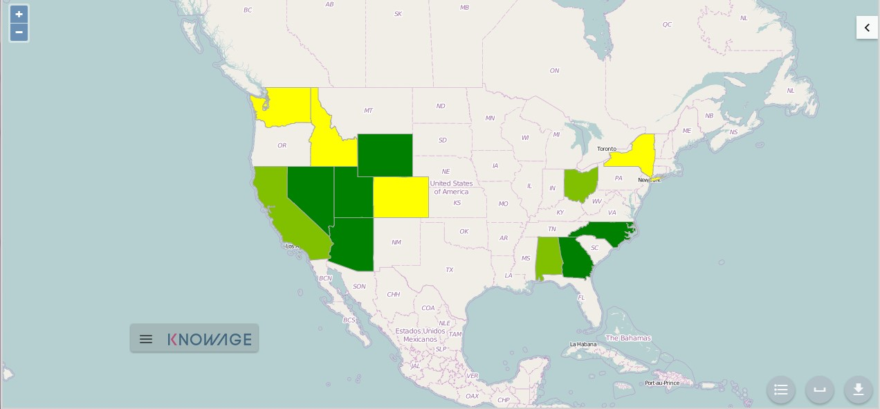
Fig. 382 Example of GIS document. USA sales per store
Click on the arrow on the top right to open the Location Inteligence options panel. Here you can choose the Map Type, the indicators to be displayed on the map and you can enter filters.
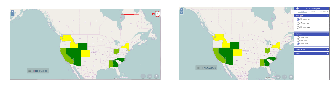
Fig. 383 Arrow button (left) Location Inteligence options panel (right) .
The Map Type available are:
- Map Zone: the different map zone are filled with different colour range according to the indicator values
- Map Point: the indicator values are displayed by points with differs on the radius. A bigger radius means a higher indicator’s value.
- Map Chart: thanks to this visualization type you can compare more than one indicators simultaneously. Choose which indicators compare among the available ones. You have to mark them in the indicator panel area to visualize them. The charts appears on the map displaying the selected indicators’ values.
These three typologies of data visualization on map are compared below.
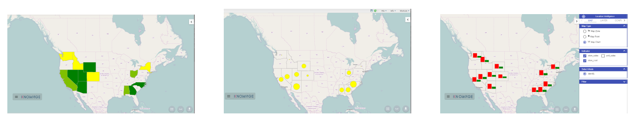
Fig. 384 Map Zone (left) Map Point (center) and Map Chart (right).
Now you can add extra layers on the default one. Switch to the layer tab of the Location Inteligence options panel.
Here click on select form catalog, choose the layers you want to add. Mark them in the bottom part of the Location Intelligence area in the Layer box and the selected layer are displayed. These steps are shown in figure below.
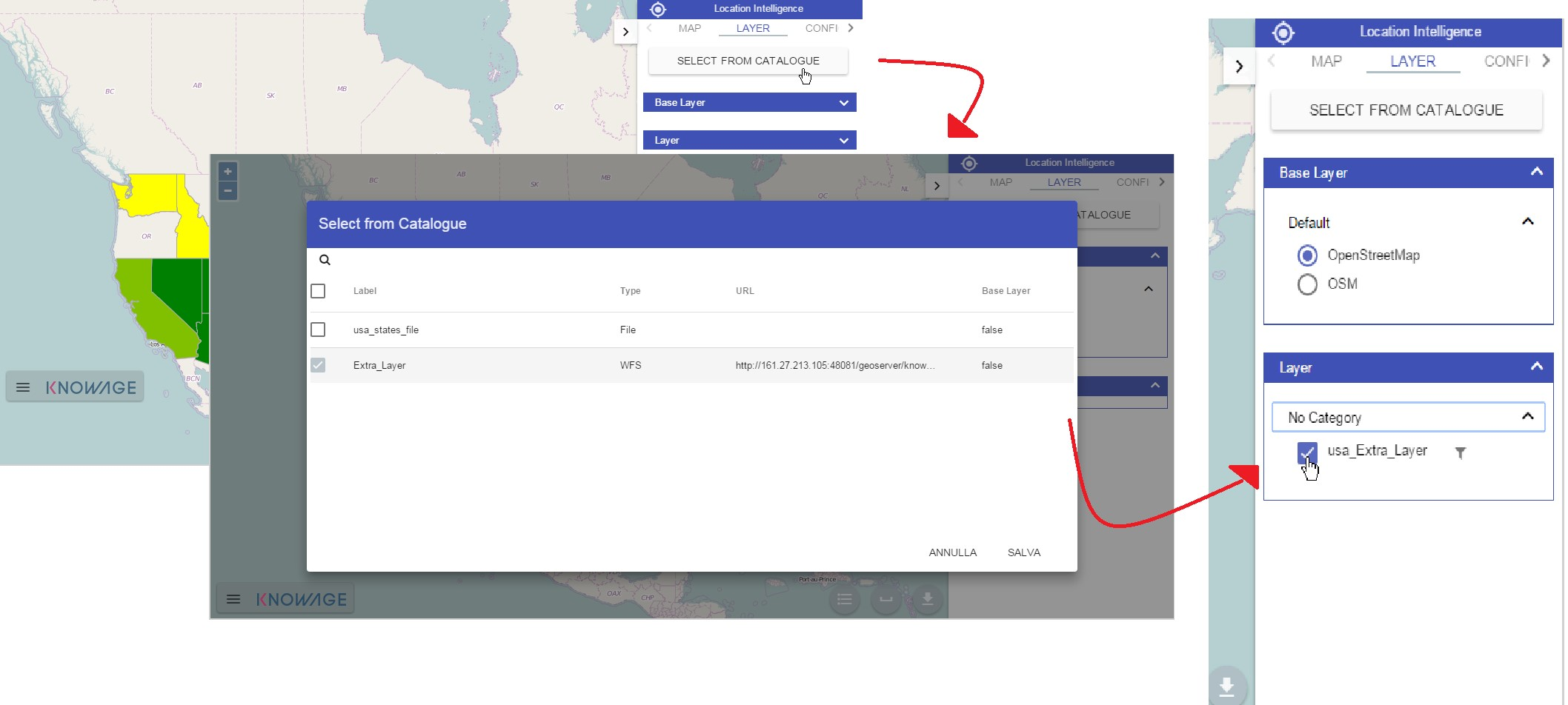
Fig. 385 Steps for layer adding
In our example we upload some waypoints, you can see the results obtained in next figure.
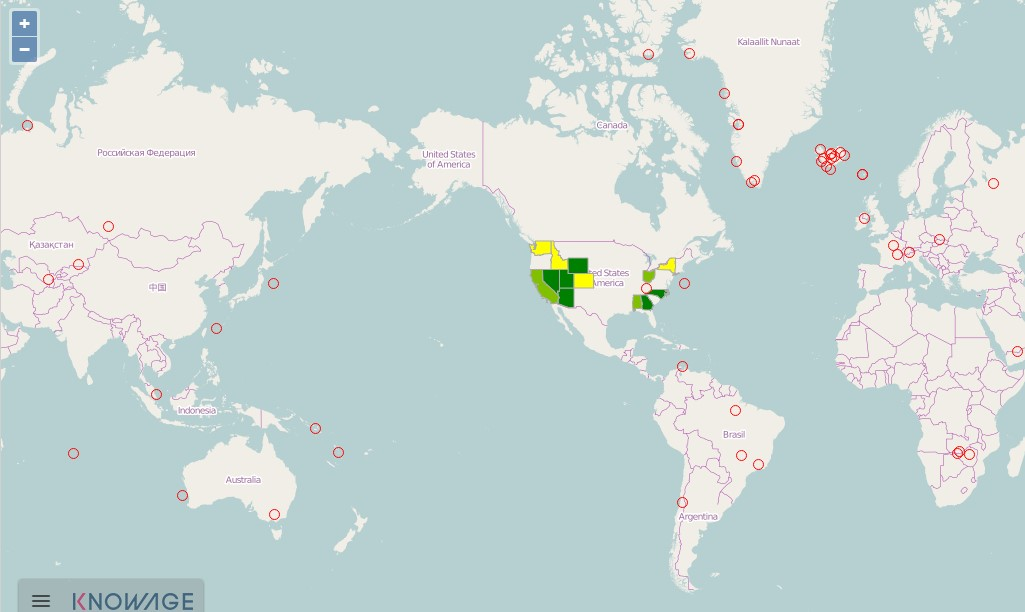
Fig. 386 Map with two layers
Now let’s focus on Configuration tab of Location Inteligence panel option. Here you can set some extra configurations. Let’s have a look them for each data visualization typology.
For the Map Zone you can set:
- Method: the available ones are quantiles or equal intervals. If you choose quantiles data are classified into a certain number of classes with an equal number of units in each classe. If you choose equal Intervals the value are divided in ranges for each classe, the classes are equal in size and their number can be set. The entire range of data values (max - min) is divided equally into however many classes have been chosen.
- N°of classes: the number of intervals in which data are subdivided.
- Range colours: You can choose the first and the last colour of the range. For both of them you can use a colour pixer by clicking on the coloured square. An example is provided below.
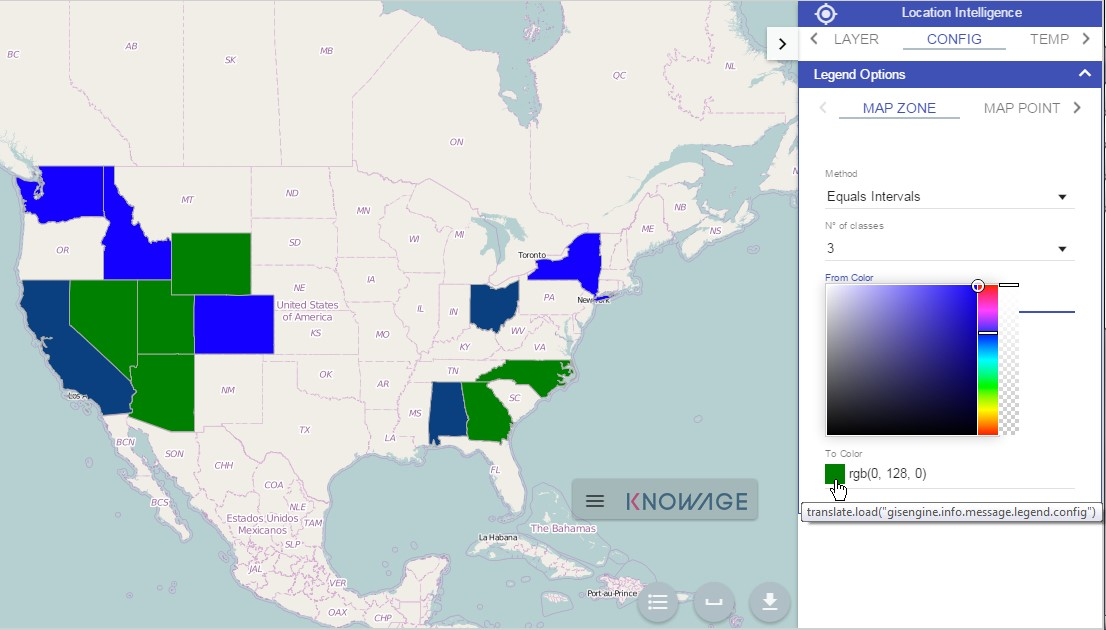
Fig. 387 Map Zone extra configurations
For the Map Point you can set:
- Colour: the colour of the circle.
- Min/Max value: the minimum and the maximum circles radius.
For the Map Chart you can set the colour of each chart’s bar.
The last tab of the panel is dedicate to the template preview, it is provided for advanced user who want to have an approach on generated code.
We can conclude our overview on GIS document describing the buttons located at the bottom right corner, you can see them underlined in the following figure. From the left to the right this bottons can be used for: have a look at the legend, compute a measure of an area of the map and do the .pdf export of the map.
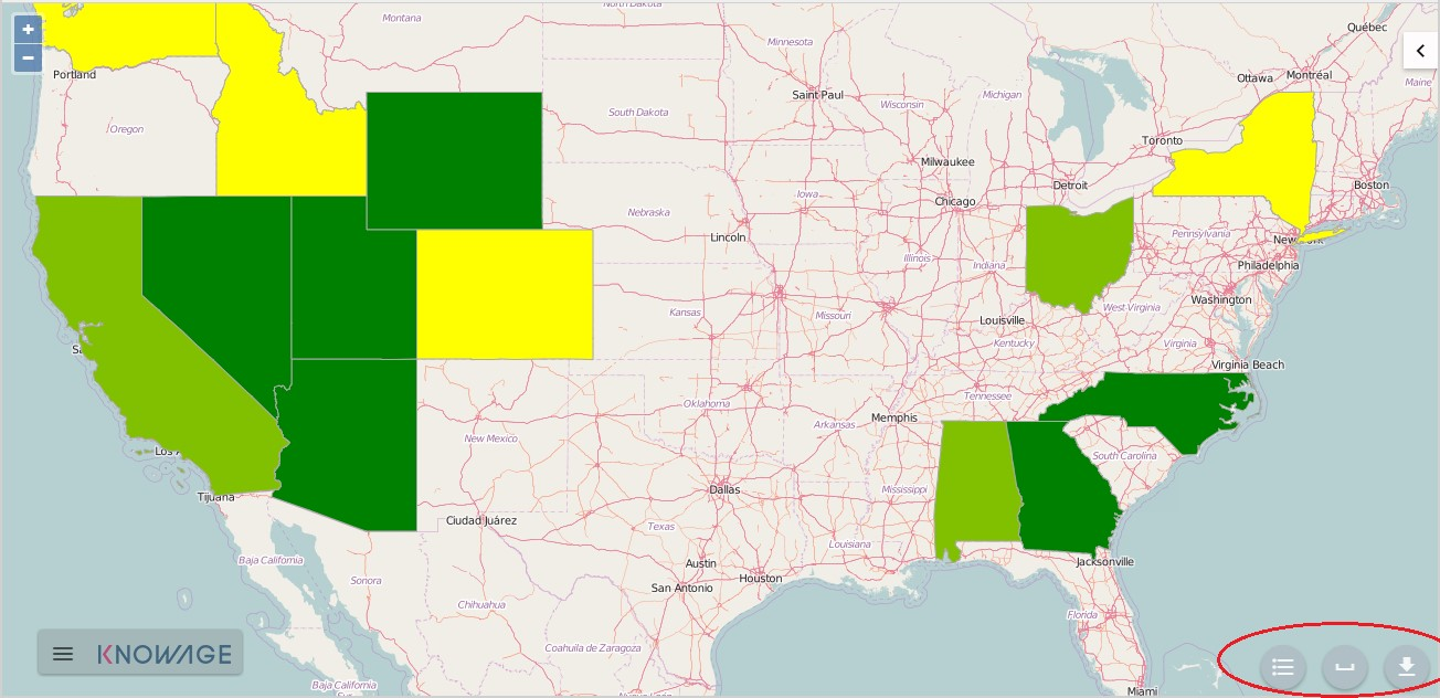
Fig. 388 From the left to the right: Legend, Measure and Export bottom.
Extra functionalities
Let’s come back to Location Layer main tab ad focus on the Select Mode area. If cross navigation has been set you find two options: identify and Cross navigation.
Select Cross Navigation, the Spatial Item tab appears. In this tab you can configure your selection. To make your selection hide CTRL key and choose the area on the map with the mouse. If you choose near, the features in the Km set are selected. If you choose intersect, the features which borders intersect your designed area. If you choose inside, only the features completely inside your area of selection are considered for the cross navigation.
When selection is made, a box appears. In this box you find cross navigation information. The number of features selected and a botton to perform the cross navigation with the active selection.
Template building with GIS designer
GIS engine document templates can now be built using GIS designer. Designer is available from administrator document detail page (for this part refer to Section 15.8) and also for end users workspace. The creation process and designer sections are described in the text below.
A GIS document can be created by a final user from workspace area of Knowage Server. Follow My Workspace » Analysis and click on the “Plus” icon available at the top right corner of the page and launch a new Geo-referenced analysis.
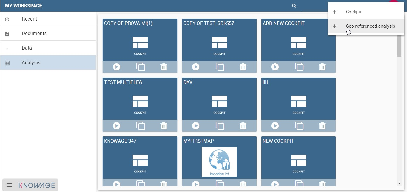
Fig. 389 Start a new Geo-referenced analysis.
When the designer is opened there is option to choose dataset for joining spatial data and business data. When the dataset is selected the Dataset join columns and indicators sections will appear. By default dataset is not chosen and there is interface to create map without business data
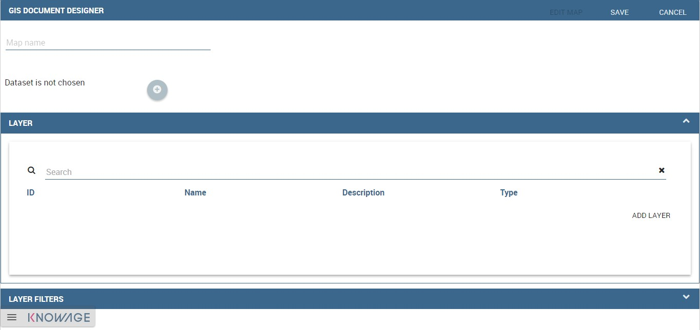
Fig. 390 GIS document designer window.
Designer sections
Layer section
Definition of the target layer is configurable in layer section. If the dataset is selected one of the available layers is chosen from list of layers catalogs. Button change layer (next figure) opens a pop up with a list of all available layer catalogs. Selecting one item from the list and clicking save the selected item will be chosen for template.
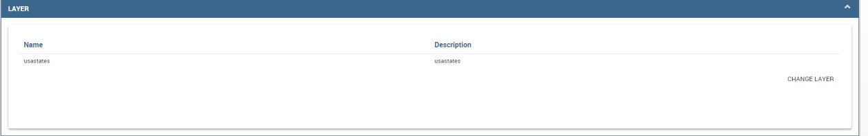
Fig. 391 Target layer definition.
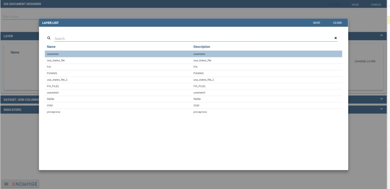
Fig. 392 List of available layer catalogs.
In case when there is no dataset multiple layers can be selected below.
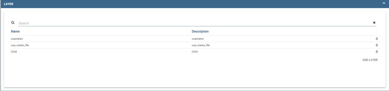
Fig. 393 Multiple selection of available layers.
Dataset join columns
Dataset join columns section is for configuring joining spatial data and business data. This section is only present when the dataset is selected for the document. Designer data structure for joining is represented by the pairs of dataset columns and corresponding layer columns. Clicking on add join column that you can see in figure below new empty pair appears. Dataset join column can be selected from columns on selected dataset by choosing an option from combo box. Layer join column should be added as a free text by editing corresponding table column.
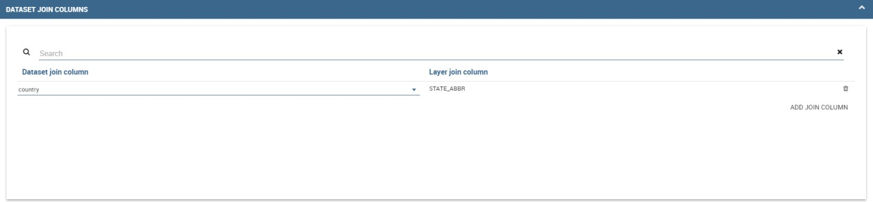
Fig. 394 Dataset join columns interface.
Indicators
Measures definition is configurable by adding indicators. The interface is shown below. This section is only present when dataset is chosen for the document. Indicators are represented by pairs of measure field from selected dataset and corresponding label that will be used on map. Clicking on add indicators creates empty pair. Measure filed should be selected by picking one option from combo box that contains measure fields from selected dataset. Label should be inserted as free text by editing corresponding table column.
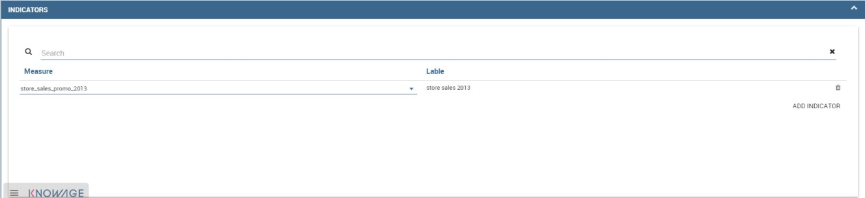
Fig. 395 Indicators interface.
Filters
Using the filtering dedicated area, as ahown in figure below, you define which dataset attributes can be used to filter the geometry. Each filter element is defined by an array (e.g. name : “store_country”, label:”COUNTRY”). The first value (name : “store_country”) is the name of the attribute as it is displayed among the properties. The second one label: “COUNTRY” is the label which will be displayed to the user. This section is only present when dataset is chosen for the document. Clicking on add filter creates empty pair. Label field should be selected by picking one option from combobox that contains attribute fields from selected dataset. Label should be inserted as free text by editing corresponding table column.
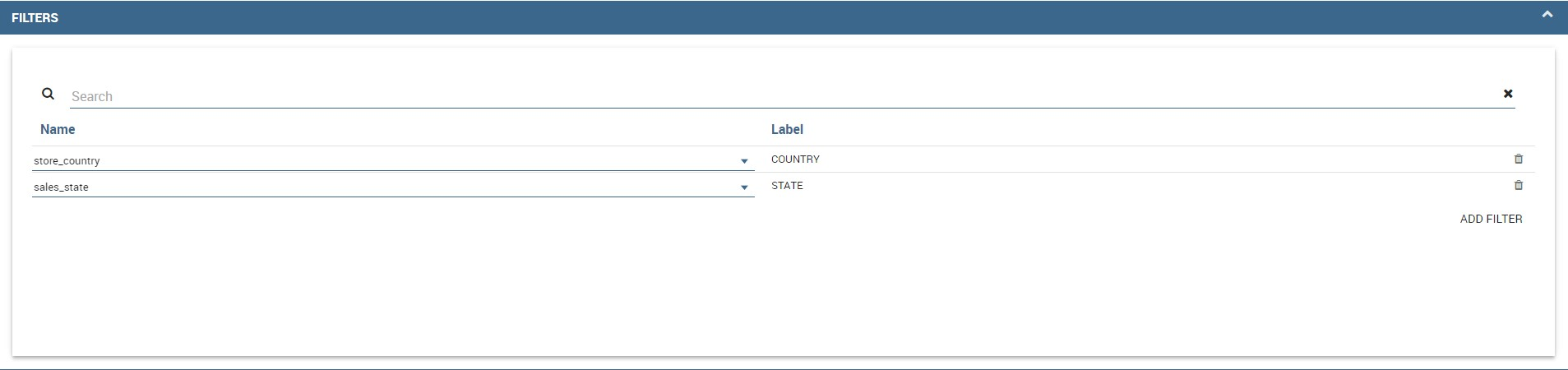
Fig. 396 Filters interface.
Map menu configuration
Through the Map menu configuration panel the user can desides to enable or disable some available functions and features, like the legend, the distance calculator and so on. See next figure to have a glimpse at the available items.
Fig. 397 Map menu configuration.
Layer filters
Here, as you can see from figure below, you define which target layer attributes can be used to filter the geometry. This section is only present when a dataset has been selected. Add filters button opens pop up where you can choose all available filters of the selected layers. Figure below gives an example.
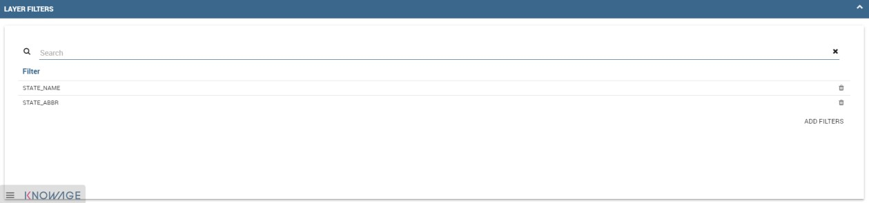
Fig. 398 Layer filters interface.
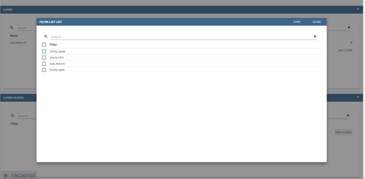
Fig. 399 List of available filters.
Edit map
When all required fields are filled basic template can be saved. From workspace user is first asked to enter name and description of new created document as in the following figure. When the template is saved successfuly EDIT MAP button is enabled in the right part of the main toolbar.
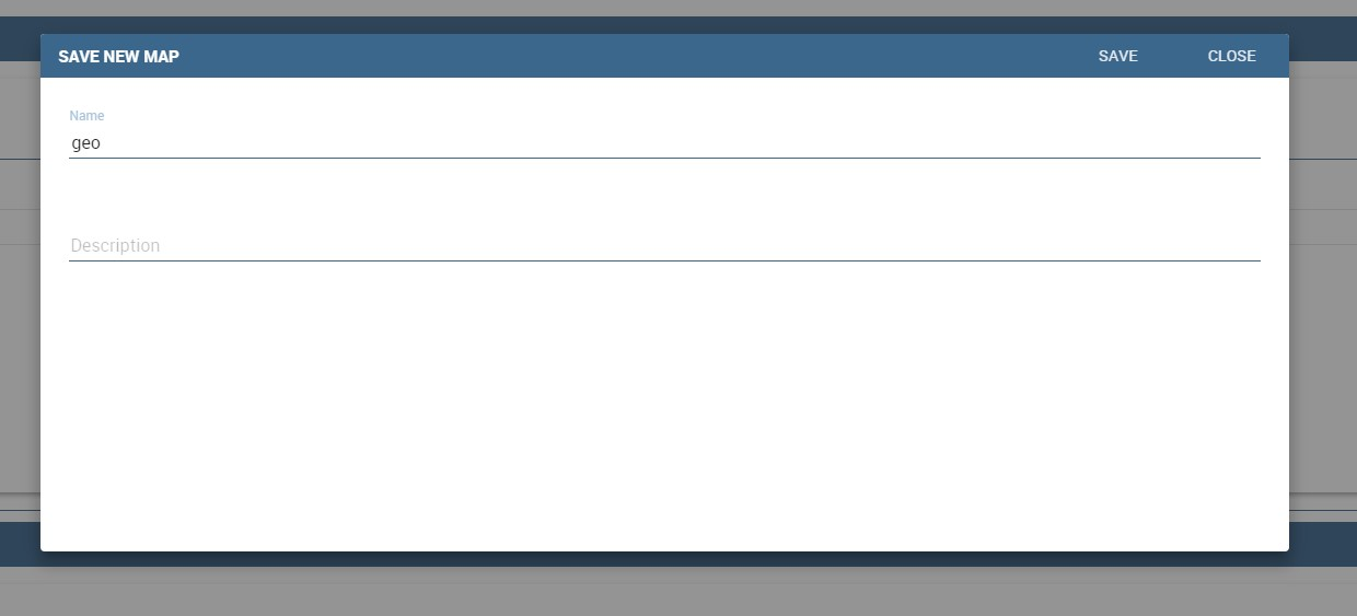
Fig. 400 interface for name and description of new geo document for end user.
Clicking the edit map button will open created map. An example is given below. In edit mode you are able to save all custom setting made on map.
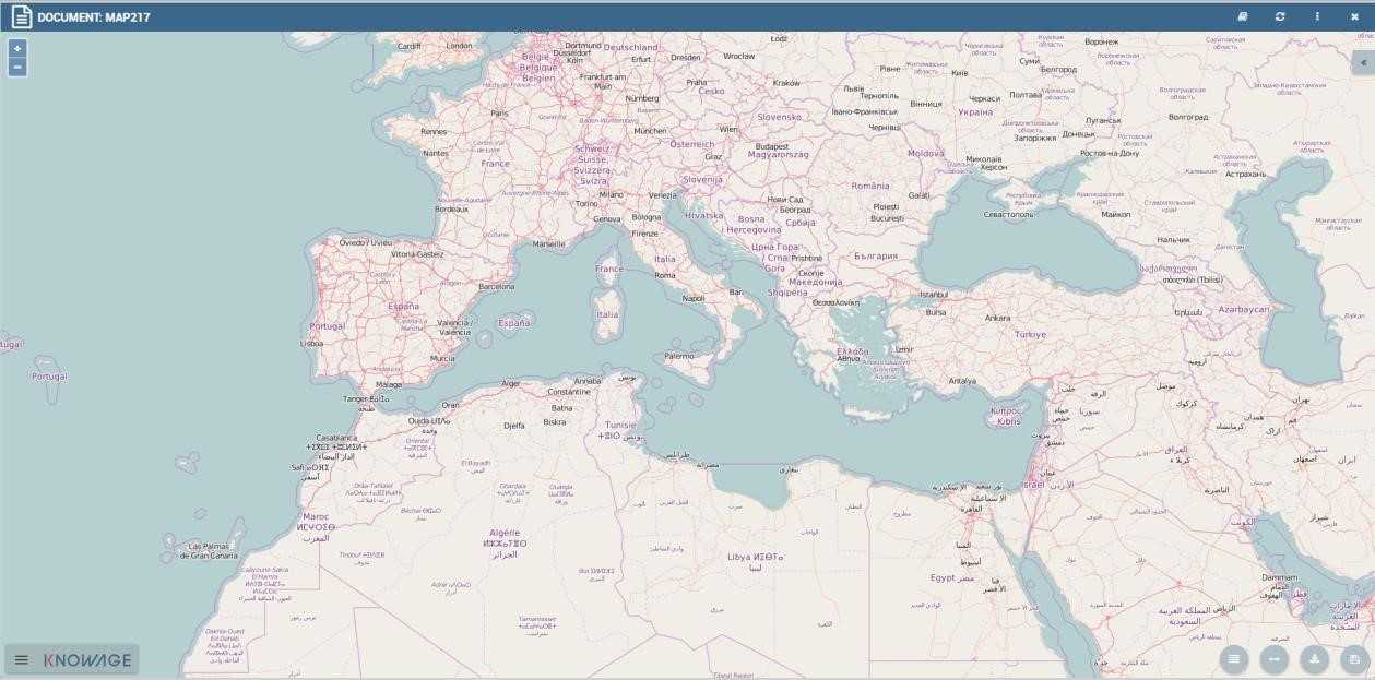
Fig. 401 Map in edit mode with save template available.
GEOReport Engine*
The GEOReport Engine implements a bridge integration architecture.
Generally speaking, a bridge integration involves both the BI and the GIS systems, still keeping them completely separated. The integration between spatial data and business data is performed by a dedicated application that acts as a bridge between the GIS and the BI suite. This application extracts the spatial data from the GIS system and the business data from the BI suite, to answer the users’ requests. Afterwards, it joins them and provides the desired results.
In particular, the GEOReport Engine extracts spatial data from an external GIS system and join them dynamically with the business data extracted from the Data Ware House, in order to produce a thematic map, according to the user’s request. In other words, it acts as a bridge between the two systems, which can consequently be kept totally decoupled.
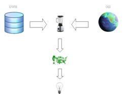
Fig. 402 Bridge integration architecture of the GEOReport Engine.
The thematic map is composed of different overlapping layers that can be uploaded from various GIS engines at the same time. Among them just one layer is used to produce the effective thematization of the map: this is called target layer.
You can manage your layers inside the Layers Catalogue.
Here you can upload the following layer types:
- File;
- WFS;
- WMS;
- TMS;
- Google;
- OSM.
Create a new layer clicking on the dedicated plus icon. On the right side you are asked to fill few settings before saving the new layer. Among these settings the firsts are equals for all types of layers. Once you choose the layer type, instead, some fields may change. This happens to manage all layers types from the same interface. For example if you choose File as type you have the possibility to chose your own .json file and upload it. After having done this, the path where your file is been uploaded is shown among the setting.
If you chose WFS or WMS you are asked to insert a specific url.
At the bottom part of layer configuration you can manage the layer visibility. Mark the role you want to give visibility previlegies on this layer. If none is marked, the layer is visibile to all role by default.
Once you have set all layer configuration you can switch to filter setting. Click on the tab you can find in the upper part of the screen, see the following figure.
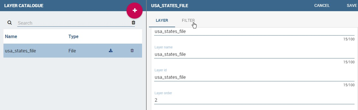
Fig. 403 Filter tab
Here you can choose which filters will be active during visualization phase. Choose among the properties of your layer, the available ones are only the string type.
Now you need to have a well-configured dataset to work with the base layer. The dataset has to contain one column matching a property field as type and contents otherwise you will not be able to correctly visualize your data on the map.
For example you can use a query dataset, connected to the foodmart data source, whose SQL query is shown in Code15.1.
1 2 3 4 5 6 7 8 9 10 11 12 13 14 15 16 17 | SELECT r.region_id as region_id
, s.store_country
, r.sales_state as sales_state
, r.sales_region
, s.store_city
, sum(f.store_sales) + (CAST(RAND() \*60 AS UNSIGNED) + 1) store_sales
, avg (f.unit_sales)+(CAST(RAND()\* 60 AS UNSIGNED) + 1) unit_sales
, sum(f. store_cost) store_cost
FROM sales_fact_1998 f
, store s
, time_by_day t
, sales_region r
WHERE s.store_id=f.store_id
AND f.time_id=t.time_id
AND s.region_id = r.region_id
AND STORE_COUNTRY = 'USA'
GROUP BY region_id, s.store_country,r.sales_state, r.sales_region, s.store_city
|
Create and save the dataset you want to use and go on preparing the document template.
Template building with GIS designer for technical user*
When creating new location intelligence document using GIS engine basic template can be build using GIS designer interface. For administrator designer opens from document detail page clicking on build template button (refer to next figure). When the designer is opened the interface for basic template build is different depending on if the dataset is chosen for the document or not.
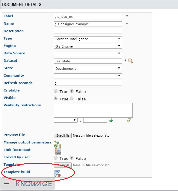
Fig. 404 Gis designer accessible from the template build.
We have already described the Gis Designer when it is accessed by a final user. Since the difference relies only in how the designer is launched we will not repeat the component part and recall to Designer section paragraph for getting details. By the way we highlight that there is a last slight difference when defining a filter on layers. In fact, using the administrator interface, if the document has analytical driver parameters, you can also choose one of the available parameters to filter the geometry, as shown below. It is not mandatory to choose layer filters so you can also save the template without any filter selected.
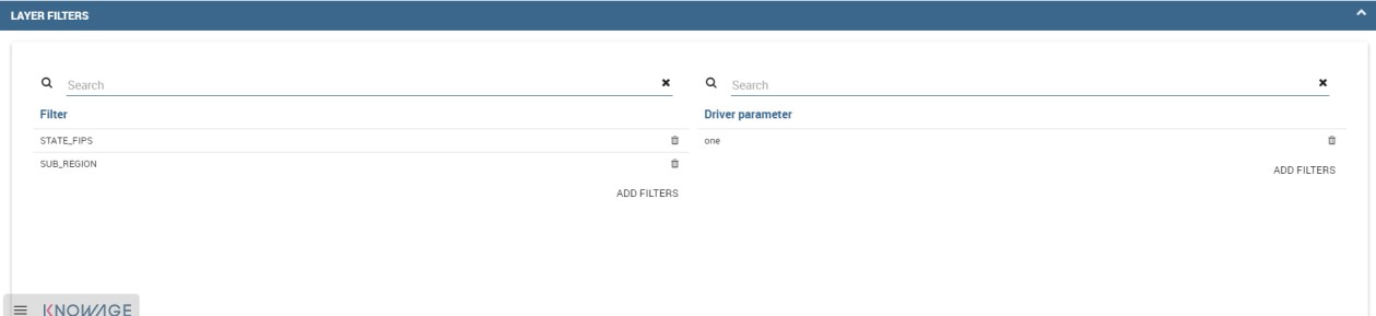
Fig. 405 Layer filters interface with analytical drivers.
When the list of selected layers is changed the filter list will be empty so you have to select filter list after filling the layer list, this is the way designer keeps consistency between layers and corresponding filters (see next figure).
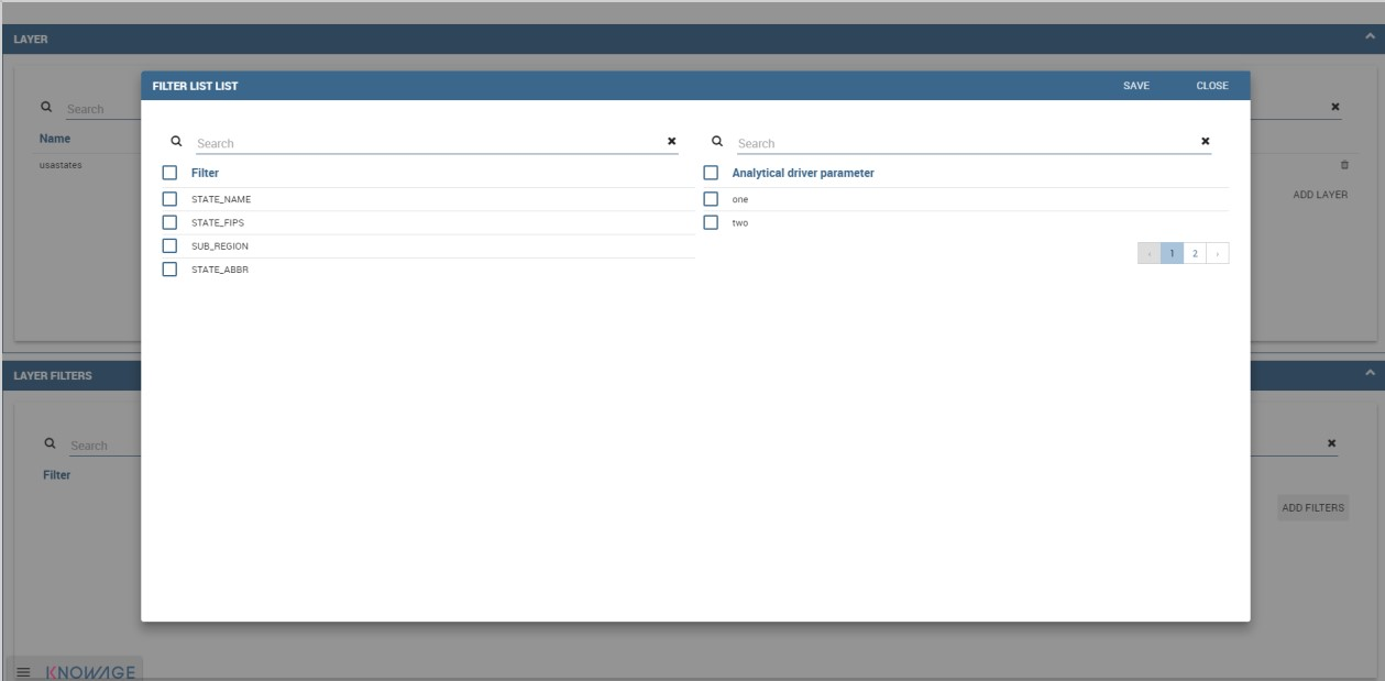
Fig. 406 List of available filters with list of analytical drivers.
Cross navigation definition*
It is possible to enable cross navigation from a map document to other Knowage documents. This means that, for instance, clicking on the state of Texas will open a new datail documents with additional information relative to the selected state.
You need to define the output parameters as described in Section Cross Navigation of Analytical Document Chapter. The possible parameters that can be handled by the GIS documents are the attribute names of the geometries of layers.
Once you have created a new Cross Navigation in the Cross Navigation Definition menu in Tools section, it is possibile to navigate from the GIS document to a target document. There is still a little step to do to activate the cross navigation.
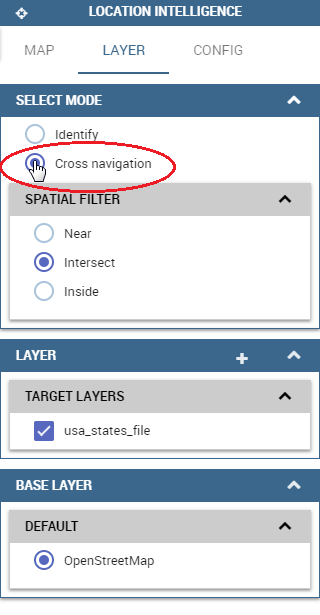
Fig. 407 Cross navigation option.
Open the layer tab of the Location Intelligence options panel and click on cross navigation select mode. Now the cross navigation is activated and if you click, for example, on one of the state it will compare the above popup.
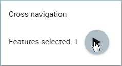
Fig. 408 Cross navigation popup.
By clicking on the play button the target document will open.